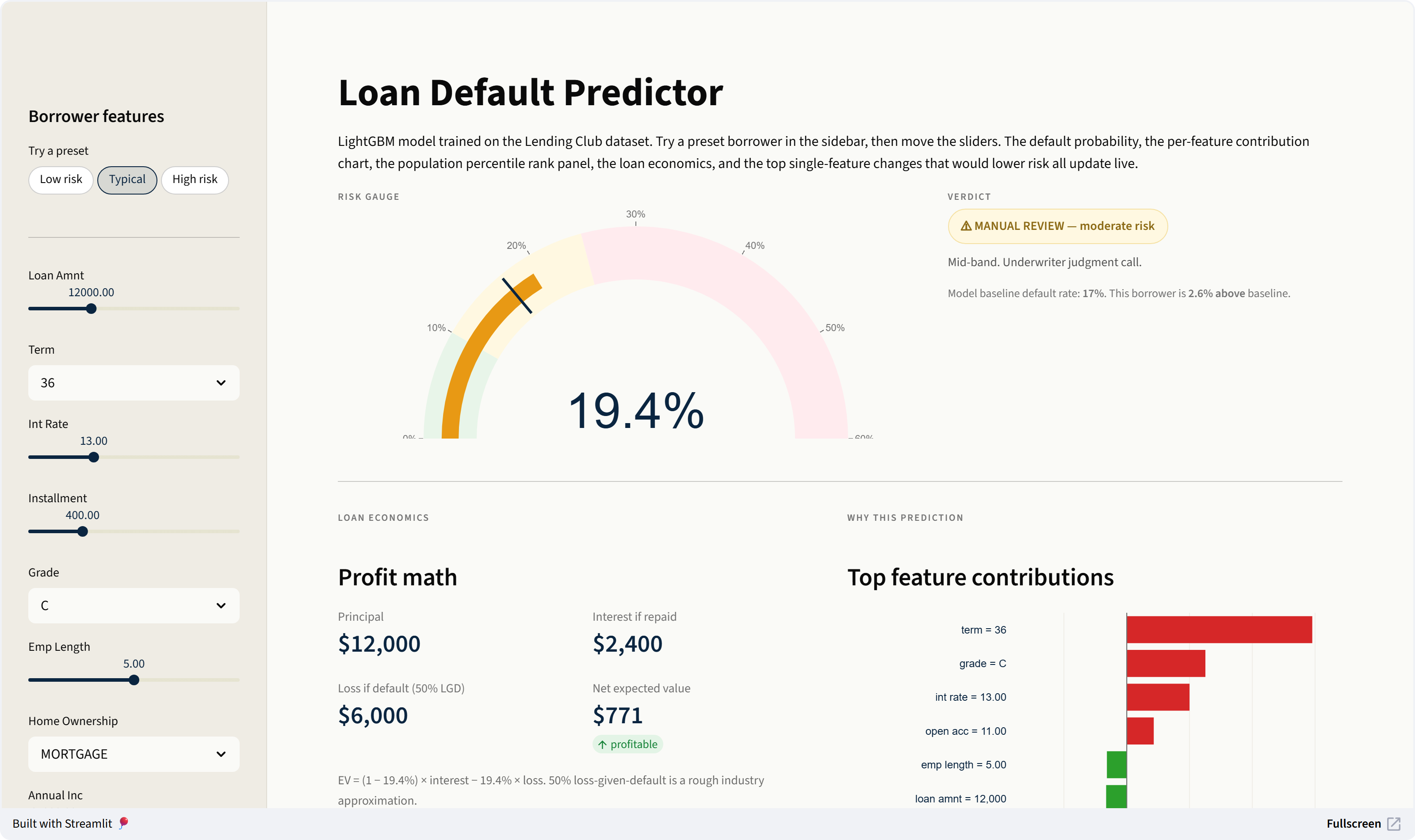
Loan Default Predictor
LightGBM model that estimates default probability for Lending Club personal loans, with a live Streamlit app you can poke at.
Why I built it
Most of my professional ML work is on regulated banking data and can't go on a portfolio. This project rebuilds the same shape of problem on a public dataset: tabular credit features at origination, gradient-boosted tree, binary default outcome.
Stack
| Layer | What |
|---|---|
| Language | Python 3.12 |
| Modeling | LightGBM 4.5 |
| Tooling | scikit-learn, pandas, numpy |
| App | Streamlit |
| Hosting | Streamlit Community Cloud |
The dataset
Lending Club's accepted-loans dataset on Kaggle. About 2.2M approved loans from 2007 through 2018 Q4, with final outcomes and the features that were known at origination. Roughly 80% paid off, 20% charged off.
Feature engineering
The whole project lives or dies here.
The leakage trap. Lending Club's data includes columns like total_pymnt, recoveries, last_pymnt_d, out_prncp. These only get populated after a loan defaults. Leave them in and the model just reads them off, "predicts" 0.99 AUC, and is completely useless on a real loan that hasn't defaulted yet. Dropping them before the model ever sees the data is the single most important thing the training script does.
Filter to settled loans. Current and In Grace Period rows go in the bin. We don't know yet what happened to them, so they're noise.
Parse the text-encoded numerics. Lending Club stores term as "36 months", int_rate as "13.5%", emp_length as "10+ years". Cast to numbers up front.
Twenty features kept, all known at origination: loan amount, term, interest rate, FICO range, DTI, employment length, home ownership, purpose, state, and the usual credit-history columns.
Subsample to 10%. Around 135K rows is more than enough. Full data trains ten times slower and the AUC barely budges.
Modeling
LightGBM classifier, 500 trees, learning rate 0.05, num_leaves 63, early stopping on validation AUC. Categoricals (term, grade, home ownership, verification status, purpose, state) go in raw — LightGBM handles them natively, no one-hot, no target encoding. 80/20 train/test split, stratified.
Results
| Metric | Value |
|---|---|
| AUC | 0.714 |
| Accuracy at 0.5 threshold | 0.804 |
| Test set size | 26,907 |
| Default rate (test) | 19.96% |
0.714 AUC is right where the published Lending Club work lands (0.70–0.75 is the usual range). If I were getting 0.85+ I'd assume I missed a leakage column and start over.
Plots


What I tried before settling on this model
A handful of experiments worth knowing about. The notebooks are in notebooks/.
Five models head-to-head (notebook 03). LightGBM defaults: 0.7132 AUC. CatBoost: 0.7191 (the winner, but 25-40x slower to train). XGBoost: 0.7137. Random Forest: 0.7034. Logistic regression with proper preprocessing: 0.7116 — within 0.0075 AUC of the best model. The gradient-boosting machinery barely beats a careful linear model on this dataset, which is consistent with how credit-default data tends to look — the signal is largely linear in the right features.
Feature engineering (notebook 04). Adding mort_acc, pub_rec_bankruptcies, application_type, plus derived ratios (loan-to-income, payment-to-income, credit history length): +0.0036 AUC.
Hyperparameter tuning (notebook 05). Optuna search across 15 trials on LightGBM: +0.0034 AUC over defaults.
Calibration (notebook 06). LightGBM's predicted probabilities were already well-calibrated for this data; isotonic on top didn't help. The percentages in the live demo are meaningful as-is.
Combined headroom over the deployed model: about 0.007 AUC, all within run-to-run noise. I left the deployed v1 in place. The bigger lift is in things I haven't tried yet — text features on desc/emp_title, time-aware vintage splitting, stacking — which published Lending Club work suggests are worth 0.01-0.03 AUC each.
One thing about the gain-importance chart above
It ranks addr_state near the top. Don't believe it. Gain importance just counts how often the model splits on each feature, and with 50 states LightGBM gets dozens of splits per tree from that one column. The deployed demo uses per-prediction contributions instead (LightGBM's pred_contrib, mathematically equivalent to SHAP for tree models) which shows what moved this specific borrower's prediction — much more honest than what the tree builder happened to fixate on globally.